Homework & Assignments

HW# 7 | 6 | 5 | 4 | 3 | 2 | 1

5.38

When you're calculating the phase angle $\delta$, you'll probably use Taylor's equation (5.65). Take note of his comment about using Figure 5.14: Even if $\omega=\omega_0$ you can still get the phase angle from the triangle in that figure.

With $\omega=\omega_0$, if you look at equation 5.65 to calculate the phase angle, you'll see that the denominator is 0. Two angles, $\pi/2$ and $-\pi/2$ have an undefined tangent. As Taylor points out, your phase is the same as the phase of the complex number written in "Cartesian" form as $(\omega_0^2-\omega^2) +2\beta\omega\,i$. Examining Figure 5.14, it looks like even though $\omega=\omega_0$, the phase angle should be $\delta=+\pi/2$.

CoCalc's arctan() quietly figures this out for you.

Other values...
$A=f_0/(2\beta\omega)=2$
$\omega_1=\sqrt{\omega_0^2-\beta^2}=0.995$
$B_1=0$; $B_2=(v_0-\omega A)/\omega_1=4.02$

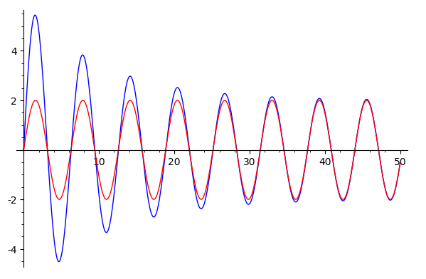
[Ebtihal] Solution in blue, attractor in red.

5.39

This one involves using CoCalc's features to solve differential equations numerically, to go directly to a numerical solution, rather than using the analytical techniques we went over in class.

Cast your eye back on what we did with numerical solutions for the skateboard on the half-pipe solution, as far as programming a second-order differential equation as 2 coupled first order differential equations.

I think I'm right about this, but check me on how to write the equation for a driven damped oscillator as a set of two coupled, first order differential equations, using the two functions $x_1(t)\equiv x(t)$ and $x_2(t)\equiv y(t)=\dot{x}_1

With the value of $\omega$ that you're using, the driving force should have a period of 1. So, to graph 5 cycles, plot $t$ on the interval [0,5].

It turns out that the numerical solution does depend on the step size you use. So pick a step size no larger than 0.01. That is...

P=desolve_system_rk4([....],[...],ics=[...],
    ivar=t, end_points=[0,5], step=0.01)

Q=[ [i,j] for i,j,k in P]
list_plot(Q,xmin=0,xmax=5,plotjoined=true)

# Or, instead of using list_plot and "joining 
# the points with lines", try this spline interpolation:
#   intP=spline(Q)
#   plot(intP,0,5)

Additionally: Try this numerical solution using two different sets of initial conditions:

1. In example 5.3, the initial conditions are $x(0)=0$ and $\dot x(0)=0$. Using these initial conditions, you should get a plot that resembles Fig. 5.15 b pretty closesly. That's your check to see that you're on the right track!
2. Now, try a different set of initial conditions: $x(0)=-1$ and $\dot x(0)=-150$. You should find that the solution starts differently, but settles down to the same "attractor" as the previous set of initial conditions.

Converting the 2nd order differential equation for the driven damped oscillator to two coupled first order differential equations. Like this: $$x_1(t)\equiv x(t)$$ $$\dot{x}_1(t)=x_2(t)$$ $$\dot x_2(t)=f(t)-2\beta x_2-\omega_0^2 x_1$$
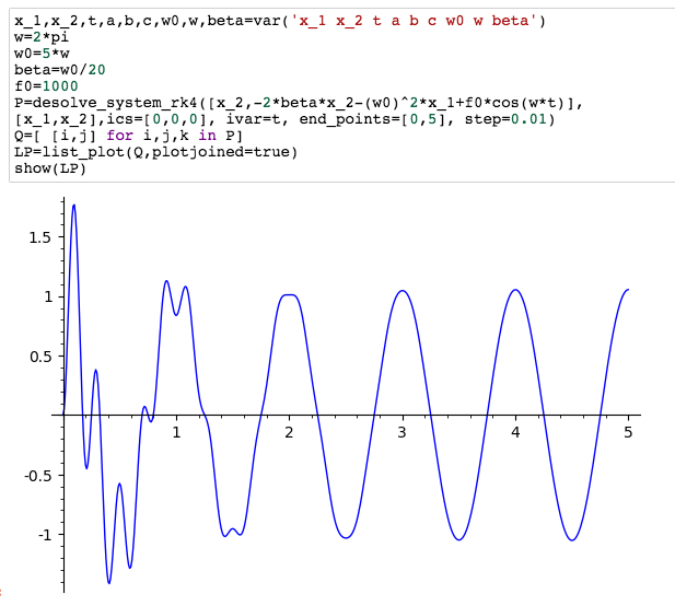
[Luke]

With initial conditions $x(0)=-1$, $\dot x(0)=-150$:

[Hugh]

5.43

Draw a force diagram to figure out the relationship between the total sinking, and the deflection (and force) of each of the four identical springs.

c.) Calculate the speed in meters/second. But also convert this to miles/hr to see if this sounds reasonable.

5.49

You should be able to write down the average value of the function ($a_0$) by inspecting the graph of the function.

6.1

One way to do this is to start with the expression for $d\myv r$ in spherical polar coordinates (equation 6 on our page about spherical polar coordinates). On the surface of a sphere, there is no change to the radius. Use this to come up with an expression for $d\myv r$ on the surface of a sphere, in terms of changes to $\theta$ and $\phi$.

6.16

7.1

The potential is $U=mgz$. So $\ddot x = \ddot y = 0$, but $\ddot z=-g$.

7.2

You should recognize the force as the same as force of a spring. To get the potential energy, remember that $\myv F=-\myv \grad U$. In this case you can probably guess the potential, and make sure your force comes out right.

The kinetic energy is $T=\frac{1}{2}m\dot{x}^2$. The potential energy $U$? Well, we know the spring force is $F_x=-kx$. But, the force is also the negative gradient of the potential energy. That is $$-\frac{\del U}{\del x}=-kx$$ The solution is $U=\frac{1}{2}kx^2+C$. But the constant drops out anyway when we take derivatives in the E-L equation. So, let's write the Lagrangian as: $$\cal L=T-U=\frac{1}{2}m\dot{x}^2-\frac{1}{2}kx^2$$ The Euler-Lagrange $\frac{\cal L}{\del x}=\frac{d}{dt}\frac{\del \cal L}{\del \dot x}$ results in .... $$-kx=\frac{d}{dt}m\dot x =m\ddot{x}$$ The solutions are... $$x(t)=A\cos\left(\sqrt{\frac km} t-\delta\right)$$ or $$x(t)=A\cos\left(\sqrt{\frac km} t\right)+B\sin\left(\sqrt{\frac km} t\right)$$ or $$x(t)=Real\left(Ae^{i\delta}e^{i\sqrt{\frac km}t}\right)$$ or several other forms...

7.3