Homework

Occasional solutions / notes

Chapter -1- | -2- | -3- | -4- | -5- | -6-

Problems in Chapter 6

HW 6.2 consists of problems 2 (i) only, 4, 8, 11(*extra credit / optional), 12, 15, 16

Problem 6.2, (i) only

This is a Gaussian wave packet. Use Desmos for the plotting parts of things. You can put in a slider for $a$.

Problem 6.4

There is a quick way to do this, by using one of our Euler identities to re-write the sin function as the sum of 2 exponentials. Oh, now try to write each of those exponentials in the form of a $\hat p$ eigenfunction, Amplitude times $e^{icx}$. What are the momenta of these two eigenfunctions?

Problem 6.8

Basically you're plotting equation 6.37. The important thing is that $\delta p \ll p_0$. I did this in Desmos, and employed a couple of different tricks to make this simpler:

• To avoid worrying about the values of the many constants, I took $m\to 1$, $\hbar\to 1$, and also $\delta p\to 1$.
• I made a slider for $p_0$, which should be large compared to $\delta p$ which is set to 1. So you might want to set $p_0$ at least to 10.
• Make a slider for time, $t$, and eventually you can switch a slider to animate that variable.
• I took the real part of the exponential in brackets. That is... $$\text{Re}\{e^{i\cdot \text{bunch o stuff}}\}=\cos(\text{bunch o stuff}).$$

Problem 6.8 animation

Problem 6.11

Extra credit! (Since I added this after assigning the homewor!) Graph the position space wave packet and animate time. This is given by eq. 6.52. Feel free to make simplifying assumptions to make the plot, similar to problem 6.8.

Problem 6.12

McIntyre has calculated the quantities $\Delta x$ and $\Delta p$ in eq. 6.60. Calculate the minimum value of the product. After that, make simplifying assumptions about the constants and graph the product as a function of $t$, but put in a slider for $\beta$ to see how that affects things. Can you understand this behavior qualitatively, taking into account the meaning of $\beta$ in terms of the range of momenta in the Gaussian packet??

Problems in Chapter 5

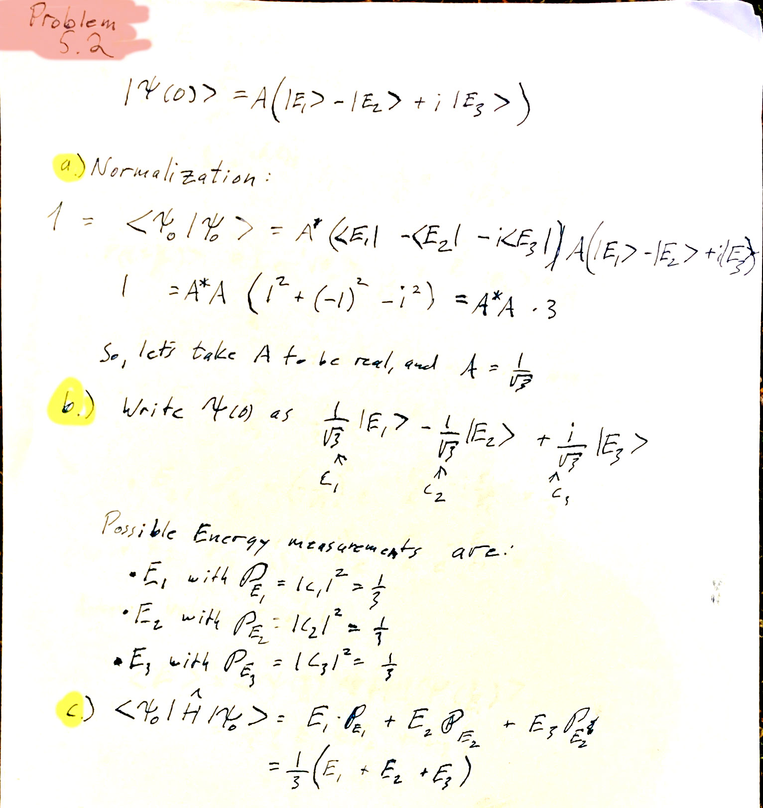
Problem 5.2

In this problem, you're working with some energy eigenstates of a Hamiltonian. The energy eigenstates are labelled with the value of their energy eigenvalue in their eigenvalue equation. That is: $\ket{E_2}$ is an eigenstate satisfying: $$\hat H\ket{E_2} = E_2\ket{E_2}.$$ The eigenstates of any observable operator (such as $\hat H$) are mutually orthogonal, and let's assume that they are also normalized to 1, such that: $$\innerp{E_i}{E_j}=\delta_{ij}.$$ They also form a complete basis, such that any state can be written as a superposition of the eigenstates: $$\ket\psi = c_1\ket{E_1} +c_2\ket{E_2} +c_3\ket{E_3} +c_4\ket{E_4}+...$$ where the constants, $c_i$, can be complex numbers.

c) Figure out the average value of the energy at $t=0$. The average value of the energy is the same as the expection value: $$\bra{\psi}\hat H\ket{\psi}.$$

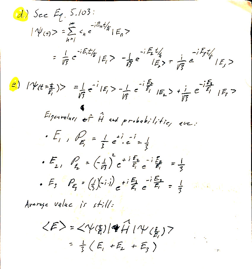
d) The time dependence in this problem is the same as what we calculated, [3.2], for kets. The first two pages of section 5.7 is a review of those results.

e) Once you've calculated what they ask, you will have enough information to calculate the average energy, at this later time. Calculate that average energy. If this quantity represents the "total energy" of the system, would you expect that to be changing with time?

Problem 5.4

Problem 5.5

See equation 5.14 for the momentum operator.

The problem is asking for a general formula for any of the eigenstates. So, you'll calculate the expectation values using the formula (involving $n$) of the eigenstates.

Eventually, the idea is to test Heisenberg's uncertainty principle, which claims that: $$\Delta_x\Delta_p \geq \frac12 \hbar.$$

Problem 5.6

It's important to evaluate your answers to this one numerically, because then you can make comparisons and do sanity checks. For example:

• If you sketch out the probability density $\phi_2(x)\phi_2(x)$ you can tell visually exactly what the answer should be.
• Since this question is about probabilities, all of your answers should be numbers between 0 and 1.

Problem 5.7

Problem 5.10

"Known to be in the right half" means that you know the probability density in the left half is 0.

Problem 5.11

Problem 5.15

Additionally:After you've derived the transcendental equation, make the sort of plot I showed you in class, with a slider for $z_0$ to vary it. You can plot the two sides of the transcendental function, of the sort that McIntyre derives, with one of the functions being the circle of radius $z_0$. Additional question: With the even functions, we found that for any $z_0 \gt 0$ there is at least one solution... so there is always a bound state even for a very shallow well. Is there always a first excited state?

Problem 5.16

Modification: Just normalize the ground state of the finite well. We'd like to use the normalized function in problem 17.

Problem 5.17

Problem 5.18

Ah, the units that experimentalists use! You'll need to get familiar with eV units and find $\hbar$ in some useful units to do your calculations.

You'll need to find the energies of all the possible bound states, that is, energies less than 5 eV above the bottom of the well. There are not an infinite number

Problem 5.23

In addition to plotting each of the normalized wave functions, also make plots of the probability density function, $\psi^*(x)\psi(x)$, for each wave function. Then you can compare the areas under the graphs for $0\lt x \lt 1$ visually among the different functions to the numbers you calculated for those probabilities.

Problem 5.24

Problems in Chapter 4

Problem 4.1

The Quantum State $\ket{\psi}$ should be a complete description of the state of a quantum system. The question is... how to describe a system of two particles in terms of the single particle kets of the two particles?

In this section, we're interested in a state consisting of an electron (moving in one direction), and a positron (moving in the opposite direction). We're not interested in the motion, but just in the spin states of the two particles, written individually as $\ket{\psi_e}$ and $\ket{\psi_p}$.

Problem 4.2

It may be helpful to remind yourself of the way that single-particle operators interact with these two-particle wave functions. See McIntyre's equations 4.1-3.

Problem 4.4

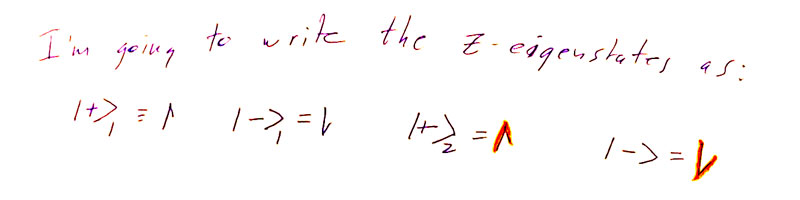
Part of the problem is just writing out all these states! I'm going to use these shortcuts for the $z$ eigenstates:
...and then I'll write out $\ket{\psi_b}$ in terms of these $z$ eigenstates, since I know the $x$ eigenstates in terms of the $z$ eigenstates. For example, a portion of this state can be written as:

You may remember that any quantum state may be multiplied by an overall phase facter $e^{i\theta}$ without changing any observable properties of the state.

We see that $\ket{\psi_b} = -1\ket{\psi_a} = e^{i\pi}\ket{\psi_a}$, so the two wave functions are equivalent.

Problems in Chapter 3

Problems 3.6, .12, .14, .15, and one of your choice

Problems in Chapter 2

Problem 2.1

It seems these "Come up with the matrix" problems do indeed require that we know the eigenstates of the operator, in the $S_z$ basis.

2.1.pdf (Calculation by hand.)

Problem 2.3

The column-vector representations of the $x$ eigenstates in the $S_x$ basis are $$\ket{+}_x\equiv\begincv 1\\0 \endcv\ \ \text{ and } \ \ \ket{-}_x\equiv\begincv 0\\1 \endcv.\label{ketxs}$$

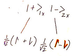
We know these two relationships between the $S_z$ and $S_x$ eigenstates: $$\ket{+}_x= \frac 1{\sqrt 2} \big(\ket + + \ket -\big).$$ $$\ket{-}_x= \frac 1{\sqrt 2} \big(\ket + - \ket -\big).$$ Solve these two equation for the two unknowns $\ket +$ and $\ket -$, in terms of the two "known" $x$ eigenstates, as written in Eq ($\ref{ketxs}$). You are finding the column vecor representations of $\ket +$ and $\ket -$ in the $S_x$ basis.

Then, once you know the column vectors for the $z$ eigenstates, you can build the matrix for $\hat S_z$, along the lines of problem 2.1.

Problem 2.7

Don't do the whole problem. I tried to solve for the eigenvectors with CoCalc. It's a little bit onerous to pick out the solutions, so I've copied out the eigenvectors below. You should check them against some ones that we know: Using Fig. 2.3, identify $\theta$ and $\phi$ for (a) $\uv n=\uv y$ and (b) $\uv n=\uv x$ and check that you get the expected column vectors for (a) $\ket +_y$ and $\ket -_y$ and (b)$\ket +_x$ and $\ket -_x$. $$\ket +_{\uv n}=k\begincv 1\\ -\frac{(\cos \theta-1)}{\sin\theta}e^{i\phi} \endcv \ \ \text{ and }\ \ \ket -_{\uv n}=k'\begincv 1\\ -\frac{(1+\cos \theta)}{\sin \theta}e^{i\phi} \endcv $$

• What you get out of Sagemath's solutions are not generally normalized to 1, so I've written the eigenvectors with constants $k$ and $k'$ which can be chosen to normalize the eigenstates for any particular choice of $\theta$ and $\phi$.
• You don't have to, but you can also check if it matches up for the $z$ eigenstates, but this involves taking some limits because the denominators blow up if you just plug in the corresponding angles...]
  Taking limits does not neatly resolve the problem. A better approach is to set $\theta=0$to make $\uv n \parallel \uv z$ and evaluate the $S_{\uv n}$ matrix (equation 2.41). Then show that $\phi$ does not appear in this matrix, and that $\ket +\propto \begincv 1\\0\endcv$ and $\ket -\propto \begincv 0\\1\endcv$ are eigenvectors of the matrix with eigenvalues $+\hbar/2$ and $-\hbar/2$.

Problem 2.8

Use the (normalized) eigenstates above, if they check out!

P.S. The eigenvectors are given in (2.42) as: $$\ket +_n =\cos \frac{\theta}2\ket + + \sin \frac{\theta}{2}e^{i\phi}\ket -$$ $$\ket -_n =\sin \frac{\theta}2\ket + - \cos \frac{\theta}{2}e^{i\phi}\ket -$$

Problem 2.14

You may do only the explicit matrix calculation. You don't need to do the second way.

According to 2.20, $$ \hat S^2\ket{sm} = s(s+1)\hbar^2\ket{sm},$$ independent of the $m$, the $S_z$ quantum number. The total spin quantum number is $s=1\Rightarrow s(s+1)=2$. So, we'd expect $$\hat S^2 ={\color{blue}2\hbar^2 \large{\mathbb{1}}}$$.

Problem 2.15

You can use the fact that the probabilities of all outcomes sum to 1 in order to calculate the last probability.

Problem 2.17

Problem 2.22

Let's say that $\P_1(\theta)$ is the probability that particle originally in the $\ket +$ state makes it through the spin up channel of the $S_{\uv n}$ analyzer. The probability depends on the setting of the $\theta$ angle of $S_{\uv n}$. You should graph $\P_1(\theta)$ to see if it makes sense.

Similarly, graph $\P_2(\theta)$, which is the probability that a particle in the spin-up state emerging out of the $S_{\uv n}$ analyzer makes it through the $\ket -$ channel on the last $Z$ analyzer.

Problem 2.23

You may use CoCalc. In order to use symbols in your calculations, declare them first as variables, e.g. var('a1 a2 a3').

Problems in Chapter 1

In the two-state problems, we can assume $(\P_{-})_{z,x,y}=1-(\P_{+})_{z,x,y}$. So it's enough to calculate $\P_+$.

Problem 1.6

Problem 1.6

$$\ket \psi = \frac 2{\sqrt{13}}\ket +_x +i\frac 3{\sqrt{13}}\ket -_x.$$

Part b: Hint: Stay in the $\ket{\pm}_x$ basis.

1.10

Note that $\ket +_y=\frac{1}{\sqrt 2}\begincv 1\\i \endcv$, so in matrix terms,
${}_y\bra +=(\ket +_y)^\dagger = (\ket+_y)_T^*=\frac{1}{\sqrt 2}\begincv 1& {\color{red}-}i \endcv$.