Partial derivatives and path independence
 ...or, how what you learned in Calc III connects to Thermodynamics!
Partial derivatives
The rules for taking partial derivatives of a function $f(x,y)$ of two independent variables, $x$ and $y$
- To find $f_x$, regard $y$ as constant, and differentiate $f(x,y)$ with respect to $x$.
- To find $f_y$, regard $x$ as constant, and differentiate $f(x,y)$ with respect to $y$.
Carter emphasizes this business of holding the other independent variable constant by sometimes writing a partial derivative like this: $$\left(\frac{\del f}{\del x}\right)_y$$ This means, take the partial derivative of $f$ with respect while holding $y$ constant.
Solve the ideal gas law for $P$ to express $P(V,T)$, and find $$\left(\frac{\del P}{\del T}\right)_V$$
This notation is usually not necessary. You should always hold all the other independent variables constant in order to find a partial derivative. But in this case it helps emphasize the perspective that we're considering $P$ to be the function, and $T$ and $V$ are treated as independent variables.
The linear approximation
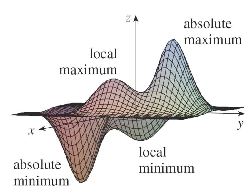
Consider the function $f(x,y)$ which can be represented as a surface in 3-d space: $f(x,y)$ is plotted as the $z$ coordinate above a particular $(x,y)$ pair.
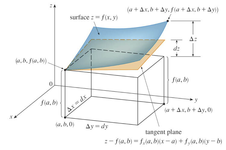
The Linear approximation for a function $f(x,y)$ of two variables, is an approximation for the change of the height of the surface, $df$, when you change $x$ by an amount $dx$, and change $y$ by an amount $dy$:
Linear approximation or (Helrich) the "Pfaffian" of $f$: $$df = \frac{\del f}{\del x}dx+\frac{\del f}{\del y} dy$$
Clairault's theorem
Suppose $f$ is defined[*] on a disk $D$ that contains the point $(a,b)$. If the functions $f_{xy}$ and $f_{yx}$ are both continuous on $D$, then $$f_{xy}(a,b)=f_{yx}(a,b).$$ [*] for $f$ to be defined it must have a uniquely determined value for every point on the disk.
Paraphrasing, I demonstrated that this meant the $xy$ "twist" of the surface in an small neighborhood has to match the $yx$ twist in order for the surface to be continuous.
And in particular, if we have a smoothly varying function on a larger region it must obey $$\frac{\del}{\del y}\left(\frac{\del f}{\del x}\right) =\frac{\del}{\del x}\left(\frac{\del f}{\del y}\right).$$ ...or For a smoothly varying, continuous function, the order of differentiation does not matter".
Path independence
If we think of $f(x,y)$ as representing the altitude of Earth's surface above sea level as a function of latitude ($y$) and longitude ($x$) as in this contour map
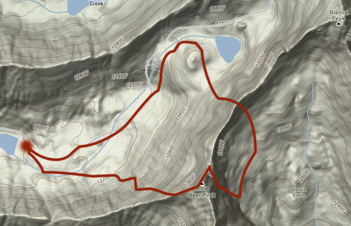
Then for some hike that we take around this landscape, along a particular path on the contour map, our net change in height, $\Delta f$, can be calculated as this path integral
$$\Delta f=\int_{\cal P} df$$
What is your net change in height/altitude if your hike begins and ends at the same point on the graph, for example, along the path above?
If the path integral around **any** closed path is $\oint df =0$, then in the language of thermodynamics, we say $df$ is an exact integral.
And in order to calculate the change of $f$ along a non-closed path, all we need to know are the values of the function at the starting and ending points: $$\Delta f = \int_{\cal P}df = f(x_f,y_f)-f(x_0,y_0).$$ We do *not* need to know the details of the path taken!
The contour map is an example of a continuous surface that could be represented by a (complicated!) function.
Here is a picture of a continuous surface which can *not* be represented as a function of $x$ and $y$. Why not??
an Equation of State
The temperature $T$ of an ideal gas in a cylinder
is a well defined function of $P$ and $V$, and can be
figured by solving the ideal gas law,
$$T(P,V)=\frac{PV}{nR}.$$
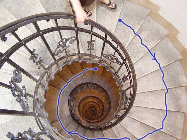
If we mess with the piston, and the temperature of the heat bath, we can move
the state of our ideal gas to different positions on a $P-V$ diagram. But if
we manage to return to the original pressure and temperature, we find that
we once again have the same temperature as when we started out.
Same behaviour as the height as you move around a contour map!
So, the fact that $dT$ is an exact differential is a consequence of the existence of an equation of state.
Equation of state
 Let each thermodynamic parameter used to specify the thermodynamic state be
one dimension of a "state space". We
can plot the thermodynamic state of the system as a point in this $n$-dimensional
space.
Let each thermodynamic parameter used to specify the thermodynamic state be
one dimension of a "state space". We
can plot the thermodynamic state of the system as a point in this $n$-dimensional
space.
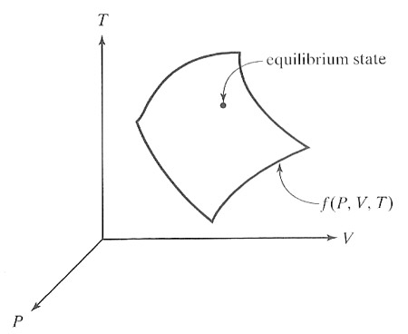
The allowed state points are not randomly distributed in this 3 dimensional space, but are "next to" each other, so as to form a surface.
If the parameters are pressure $P$, volume $V$, and temperature $T$, then there exists a functional relationship between them written as $$f(P,V,T) = 0.$$
This reduces the number of independent variables (degrees of freedom) from 3 to 2.Kerson
Huang (in "Statistical Mechanics") writes:
"In the macroscopic domain...thermodynamics is both powerful and useful. It enables one to draw rather precise and far reaching conclusions from a few seemingly commonplace observations. This power comes from the implicit assumption that the equation of state is a regular function, for which the thermodynamic laws, which appear to be simple and naive at first sight, are in fact enormously restrictive."
In Thermodynamics we will frequently take advantage of path independence even if we don't know what the equation of state is!
Test for exact / inexact differentials
 So, if someone on the street tries to sell you an exact differential...
$$dz=y\,dx-x\,dy.$$
So, if someone on the street tries to sell you an exact differential...
$$dz=y\,dx-x\,dy.$$
Test it to see if it obeys Clairault's criteria for a regular function...(the 'curl' test).
*If* $dz$ is, in fact, an exact differential, then it could be written as a Pfaffian: $$dz = \frac{\partial z}{\partial x} \, dx + \frac{\partial z}{\partial y} \, dy.$$ According to the salesman, $\frac{\partial z}{\partial x}=y$ and $\frac{\partial z}{\partial y}=-x$.
Since the order of differentiation for $z$, *if* it's a function, would not matter, we should have... $$\begineq \frac{\del}{\del y}\frac{\partial z}{\partial x} &=\frac{\del}{\del x}\frac{\partial z}{\partial y}\\ \frac{\partial}{\partial y}y &= \frac{\partial}{\partial x} (-x)\\ 1 &= -1.\endeq$$
Oops--not true! So, this is not an exact differential, and we should really write: $$\delta z = y\,dx-x\,dy.$$ To make the connection with appendix A: Let's say that a differential $dz$ is written in terms of two functions $M$ and $N$ which depend on either or both of the independent variables as $$dz=M(x,y)\,dx+N(x,y)\,dy$$ Then the Clairault test is $$\frac{\del}{\del y}M(x,y) \stackrel{?}{=}\frac{\del}{\del x}N(x,y). $$
Problem A1-a - test for exactness (2.5 min).
Integrating an exact differential
Here are my Calc III notes on a "recipe" to find the potential function.
And here's an example...
Problem A1-a Integrating $dz$ to find $z(x,y)$ (7 min).
But if you try the same kind of test on:
$$dw=\frac{\delta z}{y^2}=\frac{y\,dx-x\,dy}{y^2},$$
you should find that it passes. (A possible function is $w=x/y$). We conclude that $dw$ is an exact differential.
So $1/y^2$ is
called an integrating factor for the expression $y\,dx-x\,dy$. There are many more integrating factors.
Read Carter's Appendix A for the following:
In Electrodynamics and Mechanics we found that these characteristics of a
conservative force $\myv{F}(\myv{r})$ each imply the others: $$\myv{F} = - \myv{\nabla} U
\iff \myv{\nabla} \times \myv{F}=0 \iff \oint_{\mathcal{P}} \myv{F}\cdot d\myv{r}=0.$$ Force is the gradient of a potential. The $x-$ and $y-$components are: $$F_x = -\frac{\partial V}{\partial x};
F_y = -\frac{\partial V}{\partial y}$$
A condition for a force to be conservative (that is, something you can derive
from a potential) is that the curl of the force has to vanish. In this case,
the 'force' only has two components, and so the curl can be considered to be
a scalar since it only ever points in the same $\uv{z}$ direction: $$ \begin{aligned}\myv{\nabla} \times \myv{F}=\begin{vmatrix} When the contour integral along any closed path $\mathcal{P}$ is zero,
that means that the integral of the potential is the same along any path. $$\begin{aligned}Integrating factors
More results
Relationship with Potential Theory
$\myv{F} = - \myv{\nabla} V $
$\myv{\nabla} \times \myv{F}=0$
\uv{x} & \uv{y} & \uv{z}\\
\frac{\partial}{\partial x} & \frac{\partial}{\partial y} & 0\\
F_x & F_y & 0
\end{vmatrix}
=\uv{z}\left(\frac{\partial F_y}{\partial x}-\frac{\partial F_x}{\partial
y}\right) = \\
= \uv{z}\left(\frac{\partial}{\partial x}\frac{\partial V}{\partial y}-\frac{\partial}{\partial
y}\frac{\partial V}{\partial x}\right) = 0
\end{aligned}$$$\oint_{\mathcal{P}} \myv{F}\cdot d\myv{r}=0$
0 = \oint_{\mathcal{P}} \myv{F}\cdot d\myv{r}
= \oint_{\mathcal{P}} \left(F_x\
dx +F_y\ dy\right)\\
\oint_{\mathcal{P}}\left(-\frac{\partial V}{\partial x}dx-\frac{\partial V}{\partial
y}dy\right) =
-\oint_{\mathcal{P}}\left(\myv{\nabla}V \cdot d\myv{r}\right) = -\oint_{\mathcal{P}}
dV
\end{aligned}$$