Speed distribution
How many particles are going how fast?
If we knew the precise statistical distribution of the speeds, we could calculate detailed material properties, such as viscosities, mean free paths, etc.
Energy is exchanged and redistributed among molecules when they collide with each other. If we consider the constraints on initial and final molecular velocities in collisions, we can guess a likely probability distribution for the velocities: This will be the Maxwell-Boltzmann distribution.
Binary collisions
Consider an ideal gas consisting of just one kind of particle, each with a mass $m$.
 If the density of molecules is low enough then we only need to worry about collisions involving two molecules at a time. That is, we'll assume that the chances of 3 or more molecules colliding at exactly the same time are much lower than 2 particle collisions.
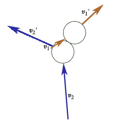
If we fix the initial vector velocities $\myv v_1$ and $\myv v_2$, are the final velocities $\myv v_1'$ and $\myv v_2'$ determined or not?
The answer turns out to be: one constraint shy of completely.
In what follows, a constraint should be thought of as a single equation that connects, typically, the $x$ or $y$ or $z$ components of the velocities.
Central forces
Assume that the forces (responsible for the change of direction during the collision) between the two particles only ever act along the line that connects them.
$\Rightarrow$ All the velocities are in the same plane.
In order to specify the velocities of both particles, both before and after the collision we need 2 components for 4 vectors = 8 numbers.
Specifying the 2 initial velocity vectors requires 4 constraints, leaving another 4 numbers free.
Momentum conservation
Momentum is conserved in the collision. The constraint that the total initial momentum is equal to the total final momentum can be written as: $$\myv v_1 + \myv v_2 = \myv v_1'+\myv v_2'.$$
Since these vectors all lie in the same plane, this amounts to 2 constraints: one for each vector component in the plane of scattering. We still have 8-4-2=2 numbers free.
Energy conservation
Assume that the collisions are elastic. The total kinetic energy before and after the collision must be the same: $$v_1^2+v_2^2=v_1'^2+v_2'^2.$$
This is only 1 constraint. So, we have 8-4-2-1=1 degree of freedom left: If the final velocities are determined, this last degree of freedom corresponds to a freedom of choice about which particle gets which final velocity.
- The final velocities *are* fully determined by the initial velocities,
- However, which particle ends up with which final velocity is *not* determined.
From this point on, we should think of the 1 and 2 subscripts as just indicating the two initial (or two final) velocity vectors to distinguish them from each other: They're no longer going to be associated with one particle or the other.
Velocity distribution function
The velocity distribution function, $F(\myv v)$ is defined such that, $$F(\myv v)\,d\myv v$$ is the number of molecules with velocities in the range $\myv v$ to $\myv v+d\myv v$.
[This is different from $f(v)\,dv$ which was the fraction of all molecules in the system with speeds between $v$ and $v+dv$.]
$aF(\myv v_1)F(\myv v_2)$
...is the number of collisions like the ones shown above in a certain time period.
The number of such collisions has to be proportional to the number of molecules
with the right initial conditions. ("$a$" is just a proportionality constant--which we will not need to calculate.)
Time reversal symmetry
Because the final velocities are uniquely determined by the initial velocities, there must be just as many collisions with final velocities $\myv v_1'$, $\myv v_2'$ as have initial velocities $\myv v_1$, $\myv v_2$.
The laws of mechanics are symmetric with respect to time. A movie of a collision, run backwards, would not violate mechanics. As long as equilibrium has been reached--and therefore entropy is not changing with time--the distribution of velocities should be the same whether the system is run forward or backward in time.
 If we run time backwards, the collisions we've been talking about look like this and now have initial velocities $- \myv v_1'$, and $- \myv v_2'$. Since the number of collisions per unit time has not changed:
$$aF(\myv v_1)F(\myv v_2)=aF(-\myv v_1')F(-\myv v_2').$$
If we run time backwards, the collisions we've been talking about look like this and now have initial velocities $- \myv v_1'$, and $- \myv v_2'$. Since the number of collisions per unit time has not changed:
$$aF(\myv v_1)F(\myv v_2)=aF(-\myv v_1')F(-\myv v_2').$$
The $a$'s cancel.
Moreover, it seems reasonable to assume that all directions of $\myv v$ (with the same magnitude $v$) are equally likely. So, we'd expect that $F(\myv v)=F(-\myv v)$, and this means... $$F(\myv v_1)F(\myv v_2) =F(\myv v_1')F(\myv v_2').$$
Taking natural logs of both sides... $$\ln F(\myv v_1) + \ln F(\myv v_2)= \ln F(\myv v_1')+ \ln F(\myv v_2').$$
If the collisions are to be elastic, that is, total initial kinetic energy = total final kinetic energy, then... $$v_1^2 + v_2^2=v_1'^2+v_2'^2.$$
The easiest way to assure that $F(\myv v)$ is compatible with this energy conservation is if: $$\ln F(\myv v) \propto v^2.$$
Since we can write $v^2=\myv v\cdot\myv v$, this could be fulfilled by: $$F(\myv v) = Ae^{-\alpha \myv v\cdot\myv v}.$$
$\alpha$ *could* be either positive or negative. But we'd like, for a probability density, that $\int_0^\infty F(\myv v)d\myv v = N$ (finite value), and if $(-\alpha)$ is a positive number, the integral is unbounded. So, we will choose $\alpha$ to be a positive quantity.
This is the Maxwell-Boltzmann distribution function
Speed distribution function
Imagine that we take all the velocity vectors for all the gas particles at one instant in time, and translate them in space so that every last one of them has their tail at the origin.
All the velocity vectors with speeds between $v$ and $v+dv$ have their tips in a thin spherical shell, which
- has a radius of $v$ from the origin,
- and has a thickness $dv$.
Assuming the velocities are uniformly distributed in direction, then the number of velocity vectors with speeds in the range $v$ to $v+dv$, which is $N(v)\,dv$, is proportional to the volume of that thin spherical shell, times the probability having a certain speed: $$\begineq N(v)\,dv &= (4\pi v^2\,dv) (F(v)) \\ \Rightarrow N(v)&= 4\pi v^2 Ae^{-\alpha \myv v\cdot\myv v}. \endeq$$
The total number of particles is: $$N=\int_0^\infty N(v)\,dv.$$
The total energy is: $$\frac{3}{2}NkT = \frac{1}{2}m\int_0^\infty v^2 N(v) dv.$$
The constant $\alpha$ can be found from the ratio of these two equations. Then, substituting $\alpha$ back into either of the two equations immediately above, the constant $A$ can be found. [Screenshot of Mathematica solution.] The result is:
The Maxwell-Boltzmann distribution, $$N(v)dv = 4\pi \left(\frac{m}{2\pi k T} \right)^{3/2}Nv^2e^{-mv^2/2kT} dv$$ is the number of molecules with speeds between $v$ and $v+dv$.
The Maxwell-Boltzmann probability distribution is: $$f_{MB}(v)=\frac{N(v)}{N}=4\pi \left(\frac{m}{2\pi k T} \right)^{3/2}v^2e^{-mv^2/2kT} $$
Using CoCalc or Mathematica, graph 3 plots of $N(v)$ in the same figure: using the values $N=1000$ and $2kT/m =$
- 0.3
- 1.0
- 3.0
You can think of these plots as showing:
- keeping $m$ fixed, how the distribution changes as you increase the temperature, $T$, of a gas of molecules with mass $m$.
- OR keeping $T$ fixed, how the distributions compare for gases, all at the same temperature, but consisting of molecules with decreasing masses.
Label each plot so we can see what temperature it corresponds to.
As you raise the temperature, you ought to have a greater number of faster molecules, and the peak of the distribution (which ought to track with the average speed) should also be moving to higher $v$-values.
Here are my graphs of $N(v)$ for $N=1000$: (Red is the lowest temperature..)
Optional: You can check your calculations by integrating $\int_0^{v_{max}} N(v')dv'=g(v_{max})$ for one or more values of $2kT/m$ above. The value of $g$ is the number of particles (out of 1000) that have a speed less than or equal to $v_{max}$. If you graph $g(v_{max})$ vs $v_{max}$, the plot ought to start at 0, and then rise and saturate at $N=1000$ as $v_{max}$ gets larger and larger.
Root-mean-square speeds
We used $f(v)$, the fraction of all molecules with speeds between $v$ and $v+dv$, to calculate things like rms speeds. $$f(v) = N(v)/N.$$
So, $$\begin{align}\overline{v^2} & = \int v^2 f(v) dv = \frac{1}{N}\int v^2 N(v) dv =\\ & = 4\pi \left(\frac{m}{2\pi k T} \right)^{3/2} \int_0^\infty v^4 e^{-mv^2/2kT} dv .\end{align}$$
See Appendix D2 for the integral: $$\begin{align}\overline{v^2} & = 4\pi \left(\frac{m}{2\pi k T} \right)^{3/2} \left[\frac{3}{8 (m/2kT)^2}\left( \frac{\pi}{m/2kT}\right)^{1/2} \right]\\ & = \frac{3kT}{m} .\end{align}$$
The rms speed is
$$v_{rms} = \sqrt{\overline{v^2}}=\sqrt{\frac{3kT}{m}} = 1.732\left(\frac{kT}{m}\right)^{1/2}.$$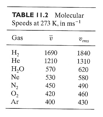
Applications
- Why don't we have more hydrogen in our atmosphere?
- Measuring isotope ratios in arctic ice cores to get at pre-historic temperatures.
- Uranium bound to fluorine as $UF_6$ is a gas. Gaseous diffusion has been used to separate the fissile uranium-235 isotope from other isotopes to make bombs.