Divergence and curl of the magnetic field
Biot-Savart = brute-force integration to get $\myv B$. Isn't there *any* other way to find the $\myv B$ field??
We've been down a road like this with $\myv E$ before:
- Coulomb's law $$\myv E(\myv r)=\int \frac{\rho(\myv r')}{\rr^2}\,d\tau'$$ = brute-force integration of the charge density to get $\myv E$.
- But we found $\myv \grad\cdot\myv E=\rho(\myv r)/\epsilon_0$, and together with Gauss' law could argue that the flux of $\myv E$ through any surface is proportional to the enclosed charge.
- And $\myv \grad \times \myv E=0$ implied that there was a scalar potential $V(\myv r)$ such that $\myv E=-\myv \grad V$.
We need to come up with two results... $$\myv \grad \cdot \myv B = 0,$$
and... $$\myv \grad \times \myv B = \mu_0 \myv J.$$
This will allow us to use Ampere's law in high symmetry cases to find $\myv B$ instead of brute force integration.
Divergence of $\myv B$
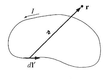 We've got a formula--the Biot-Savart law--for calculating the magnetic field from a current. We'll tweak it just a bit to write it in terms of the current density instead of a current like this:
$$\begineq\myv B(\myv r) &= \frac{\mu_0}{4 \pi} \int \frac {\myv I \times \uv{\rr}}{\rr^2} dl' \\ &= \frac{\mu_0}{4 \pi} \int \frac {\myv J(\myv r') \times \uv{\rr}}{\rr^2} d \tau' .\endeq$$
Now, let's take the divergence--wrt the unprimed components of $\myv r$: $$\begineq \myv \grad \cdot \myv B(\myv r) &= \frac{\mu_0}{4 \pi} \int \myv \grad \cdot \left(\myv J(\myv r') \times \frac{\uv \rr}{\rr^2}\right) d \tau'.\endeq$$
Using product rule 6: $\myv \grad \cdot (\myv A \times \myv B) = \myv B \cdot (\myv \grad \times \myv A) - \myv A \cdot (\myv \grad \times \myv B)$: $$\begineq \myv \grad \cdot \left(\myv J(\myv r') \times \frac{\uv \rr}{\rr^2}\right) &=\frac{\uv{\rr}}{\rr^2} \cdot \myv \grad \times \myv J(\myv r')- \myv J(\myv r') \cdot \myv \grad \times \frac{\uv\rr}{\rr^2} .\endeq$$
Now, notice that...
- $\myv \grad \times$ is operating wrt to unprimed $\myv r$ components, but $\myv J$ is a function of the primed $\myv r'$ variables, $\Rightarrow \myv \grad \times \myv J(\myv r') = 0$.
- In problem 1.62, you found that $\myv \grad \times \frac{\uv\rr}{\rr^2} = 0 $.
So both terms vanish, and we have... $$\myv \grad \cdot \myv B = 0.$$
Remember $\myv \grad \cdot \myv E = \rho/\epsilon_0$? This result for $\myv B$ is just re-phrasing an assumption that was implicitly coded into the Biot-Savart law... "There are no magnetic monopoles".
Curl of $\myv B$
Take the curl of the Biot-Savart law... $$\myv \grad \times \myv B(\myv r) = \frac{\mu_0}{4 \pi} \int \myv \grad \times \[\myv J(\myv r') \times \frac{\uv\rr}{\rr^2}\] d \tau'.$$
Handy product rule 8 says: $$\begineq\myv \grad \times (\myv A \times \myv B) &= (\myv B \cdot \myv \grad) \myv A - (\myv A \cdot \myv \grad) \myv B + \myv A \cdot (\myv \grad \cdot\myv B ) - \myv B \cdot (\myv \grad \cdot\myv A ) \endeq$$
Since that $\myv \grad$ contains derivatives wrt to unprimed components of $\myv r$, we can drop any terms containing unprimed derivatives of $\myv J (\myv r')$: $$\myv \grad \times \[\myv J(\myv r') \times \frac{\uv\rr}{\rr^2}\]= \myv J (\myv \grad \cdot \frac{\uv\rr}{\rr^2}) -(\myv J \cdot \myv \grad) \frac{\uv \rr}{\rr^2} .$$
The second term vanishes after...
- using product rule 5,
- recognizing that the divergence of $\myv J$ vanishes for steady-state currents, and
- converting a divergence to a surface integral and assuming that current densities are going to drop off to zero at infinity.
See section 5.3.2 for details!
The first divergence term is proportional to a dirac $\delta$ function, so we have... $$\myv \grad \times \myv B = \frac{\mu_0}{4\pi}\int \myv J(\myv r') 4\pi \delta^3(\myv r - \myv r') d \tau' = \mu_0 \myv J(\myv r).$$
For the electric field we had $\myv \grad \times \myv E = 0$
Ampere's law
So we had... $$\myv \grad \times \myv B = \mu_0 \myv J(\myv r).$$
Using Stoke's law, we can integrate to get... $$\int (\myv \grad \times \myv B)\cdot d \myv a = \oint \myv B \cdot d \myv l = \mu_0 \int \myv J \cdot d \myv a.$$ This is
 Ampere's law:
$$\oint \myv B \cdot d \myv l
= \mu_0
\int \myv J \cdot d \myv a.$$
The integral on the right is over an area. (It's the "charge flux".)
Ampere's law:
$$\oint \myv B \cdot d \myv l
= \mu_0
\int \myv J \cdot d \myv a.$$
The integral on the right is over an area. (It's the "charge flux".)
The integral on the left is around the path that bounds the area
Consider that $\myv J(\myv r)=\rho(\myv r)\myv v(\myv r)$, $J$ has units of charge/area/sec, and the units of $\int \myv J\cdot d\myv a$ will be Coulombs / second, the same units as "current". So that integral is the rate at which charge is passing through the surface.
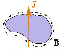
There's a right hand rule useful in defining which directions are positive:
- With your fingers curled around the closed circuit pointing in the positive direction of path integration, (same direction as $\myv B$ in the diagram),
- Your thumb points in the direction of positive $d \myv a$. (The same direction as $\myv J$ in the diagram).
Convince yourself that it doesn't matter really which orientation you choose for the positive direction of current flow, so long as you apply this right hand rule...
Using some terminology that is intentionally similar to Gauss's law...
Paraphrasing:
The path integral of $\myv B$ around a closed path
is equal to the "enclosed current" piercing (any surface) bounded by the path:
$$\oint \myv B \cdot d \myv l = \mu_0 I_\text{enc}.$$
Applications of Amperes law
Just like Gauss's law, Ampere's law is "always true and sometimes even useful". Those sometimes are generally in high-symmetry situations. For instance:
Field of an infinite wire
Consider a current $I$ flowing through a straight wire.
 If we draw
an imaginary circle (an 'Amperian loop' in analogy with a 'Gaussian surface') a constant
distance $s = |\myv\rr|$ from the wire, then by symmetry, the magnetic field
ought to have the same magnitude and orientation relative to the loop at all
points along the loop.
If we draw
an imaginary circle (an 'Amperian loop' in analogy with a 'Gaussian surface') a constant
distance $s = |\myv\rr|$ from the wire, then by symmetry, the magnetic field
ought to have the same magnitude and orientation relative to the loop at all
points along the loop.
What is that orientation? To figure that out, it is handy to remember the term in the Biot-Savart law that each piece of current contributes to the magnetic field in the direction $\myv I \times \myv \rr.$
So, apparently the $\myv B$ field is tangent to the Amperian loop shown at every point along the loop. That is, if we put a cylindrical coordinate system in:
- with $\myv I$ pointing in the $\uv z$ direction,
- $\myv B$ is pointing in the $\uv{\phi}$ direction.
- Since $\myv B$ has the same magnitude and orientation relative to the loop at all points, we can pull the magnitude of $\myv B$ out of the integral like so..
Rearranging for $B$: $$\myv B = \frac{\mu_0 I}{2 \pi s} \uv{\phi}.$$ The same result we arrived at with beaucoup de integration using Biot-Savart.
Field near a long solenoid
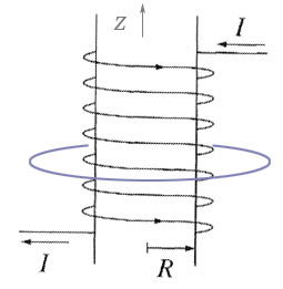
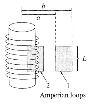
Imagine a long solenoid with many coils of wire wrapped in such a way that the current is flowing practically parallel to the $\uv{\phi}$ direction in the diagram at right. What direction is the field?
$B_{\phi}$?
If there is a $\phi$ component to the magnetic field, then for the imaginary (blue) Amperian loop shown we should have....?
$B_{s}$? -
Think of each turn of the wire as a circle of current.
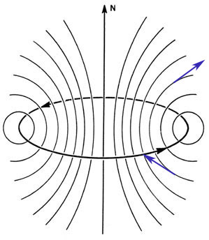
Schematically, the field of a single current loop looks something like this. We don't need to know the details, but it should be obvious that...
The radial ($\uv s$) components of
the field above and the same distance below the loop are equal and opposite.
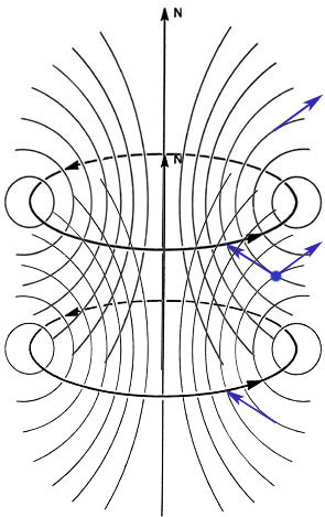
$B_{z}$?
From the two loop diagram, it looks like the field inside two loops should add up to something pointing in the $\uv{z}$ direction. What about outside the two loops?
Summarizing: $$\myv B = \begin{cases} \mu_0 n I\uv{z}& \text{ inside (along CL, far from either end)} \\ 0& \text{ outside ($s\gg r$)} \end{cases}$$