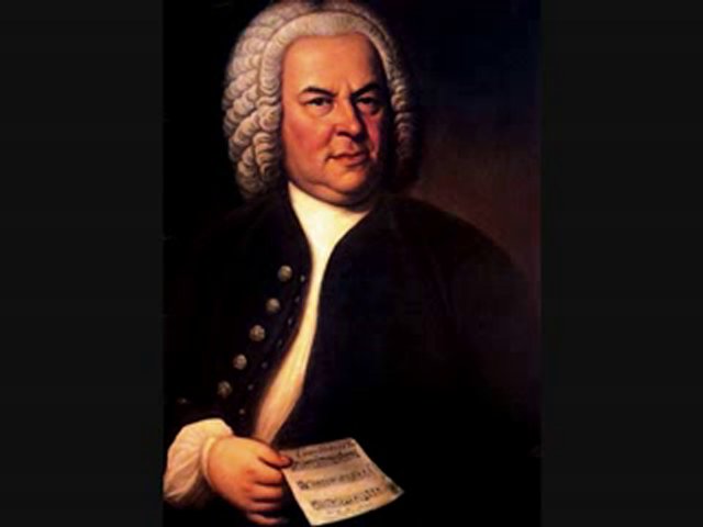
EPR and JSB
No, no, not this J.S.B. ...

Bell's inequality
Next time:
* show derivation of $\hat S_\theta$ but hide derivation of expectation value of products
* Assign them to go through the Bell paper, rather than me showing them the steps
* Correct solution to 4.50 where it's in terms of p's and e's instead of 1's and 2's.
* Show graphically limit of realism vs QM calculation
Yes, this J.S.B.
 John Stuart Bell (1928-1990) Northern Irish physicist.
The argument of E,P, and R was that we can know what $S_x$ of the positron is by measuring $S_x$ of the electron.
John Bell looked deeply at the EPR paper, and claimed that these two assumptions lie behind this argument:
- Realism: the value of a measurement on an object is objectively present in the object before the measurement is made.
- Locality: causative influences can't travel faster than light. Or objects are only influenced by things in their neighborhood (as defined as within a distance $\Delta x\lt c\Delta t$).
Bell personally, appears to have favored the EPR argument. He considered that a particle might carry with it some "hidden variables" (at least, hidden from Quantum Theory) that might determine what value would be measured depending on the setting of an S-G analyzer.
He showed that these two assumptions lead to an inequality, Bell's inequality, that any such "hidden variable" theory obeying these assumptions must obey.
It turns out that when the two detectors are equally aligned the inequality does not necessarily predict any difference between the two theories. But other sets of orientations it gets more interesting!

McIntyre considers a particular set of orientations, which are chosen at the two analyzer stations at random, and offers a straightforward way of totting up the possible probabilities for a set of hidden variables.
We consider that somehow each electron (positron) carries with it something that amounts to instructions about how it should present itself for different orientations of an S-G analyzer. We will limit ourselselves to the instructions for the three $S_{\hat n} orientations in the $x-z$ plane, which are evenly distribute, 120${}^o$ from each other. We can describe all the vectors in the $x-z$ plane with $\phi=0$ and $0 \lt \theta \lt 2\pi$
- $\hat a=\hat z \Rightarrow \theta = 0$ and $\phi=0$.
- $\hat b \Rightarrow \theta=2\pi/3$.
- $\hat b \Rightarrow \theta=4\pi/3$.
Read section 4.1 carefully
...and answer these reading questions.- On Page 100, McIntyre shows that for particles of population 2, there are nine possible outcomes. 4 of these have the same spin outcomes, and five have opposite spin outcomes.
Write out all the possible combinations for (Drew) populations 3 and 4 and (Bryan) populations 5 and 6 to verify that you also get 4 same and 5 opposite spin outcomes for each of these.
- In the lead up to equation 4.5, McIntyre is trying to calculate an overall probability by calculating a weighted average of the probabilities. The weighting factor for instruction set $i$ in table 4.1 is $N_i/\sum_i N_i$. Calculate the weighting factors for each of the 8 sets, and express them as percentages, if: $N_1=60$, $N_2=N_3=N_4=20$, $N_5=N_6=N_7=10$, and $N_8=0$.
- Equation 4.5: Why do $N_1$ and $N_8$ not appear in the first sum? Why do they appear in the second sum?
- Extreme cases: Let $N_1=90$ and all the other populations are zero. Calculate the left-hand side of both equations in 4.5 and see if the inequality holds.
- Extreme cases: Let $N_4=90$ and all the other populations are zero. Calculate the left-hand side of both equations in 4.5 and see if the inequality holds.
- Any questions or uncertainties you have about equation 4.5?
- Starting in Equation 4.7, we're using McIntyre's expression for the eigenstates of $\hat S_{\hat n}$ in terms of Spherical-Polar angles $\phi$ and $\theta$. See his equation 2.42. Questions about 4.7 or 4.9??