The Boltzmann distribution - Quantum Mechanics version
Classically, we found the probability density of speeds, $f(v)$ for the equilibrium state of an ideal gas using the assumption that $f(v)$ does not depend on time in the equilibrium state.
Quantum calculation: The energy levels of a particle in a box are quantized, and depend on the volume of the box. We will count the number states, and the degeneracy of each state. The energy of each state is the quantized kinetic energy of a point particle in a box of volume $V$.
Our story so far...
- We have a formula (complicated) for the thermodynamic probability $w_B(N_1,N_2,N_3,...,N_n)/\Omega$ of a quantum system (particles in a box). There are $n$ different energy levels.
- We need to find the most probable state (which is the equilibrium state) of the system, by varying all the $N_j$ (gulp!) subject to constraints.
- The two constraints are:
- The total number of particles, $N$, in the system is fixed.
- The total energy, $U$, of the system is fixed.
Our mission: To find that equilibrium state!
In classical thermodynamics the equilibrium state is a function of things like volume and temperature. You will not see $T$ and $V$ at first ...
But
- $U$ (one of our constraints) is a function of temperature.
- The allowed energy levels, and density of states depend on $V$.
Finding the maximum value of $w_B$
We were hoping for *some* way to maximize the function which counts the number of microstates: $$w_B(N_1, N_2, N_3...N_n) = N! \prod_{i=1}^n \frac{g_i^{N_i}}{N_i!}.$$ Gotta try varying all $n$ of those occupation number, $N_1, N_2,...$ until we find the combination that maximizes $w_B$...!
It's generally easier to maximize $\ln(w)$, which can be written as $$\ln(w_B) = \ln N! + \sum_i N_i \ln g_i - \sum_i \ln N_i!.$$
[*] It's OK to maximize $\ln(w_B)$ because $\ln(x)$ is a monotonically increasing function of $x$.
 That Scottish
mathematician (who feared
only "assassination on account of having discovered a trade secret
of the glassmakers of Venice") swoops in to profer his approximation-- $\ln(n!) \approx n\ln(n) - n$, and so...
$$\ln(w_B) = {\rm const} + \sum_i N_i \ln g_i - \sum_i N_i\ln N_i +
\sum_i N_i .$$
That Scottish
mathematician (who feared
only "assassination on account of having discovered a trade secret
of the glassmakers of Venice") swoops in to profer his approximation-- $\ln(n!) \approx n\ln(n) - n$, and so...
$$\ln(w_B) = {\rm const} + \sum_i N_i \ln g_i - \sum_i N_i\ln N_i +
\sum_i N_i .$$
Does $g_i$ depend on $N_i$?
We've got two constraints to worry about as we search for the maximum value of $\ln w_B$: $$\phi=\sum_i N_i = N; \ \ \eta=\sum_i N_i E_i=U.$$
 But Giuseppe has roused himself
from his melancholic reflections to remind us to solve a bunch of equations like $\frac{\partial f}{\partial x_i} +\alpha\frac{\partial \phi}{\partial x_i}
+\beta\frac{\partial \eta}{\partial x_i}
= 0$. Translating into our context, we have to solve $n$ equations, like
$$\frac{\partial \ln w_B}{\partial N_j} +\alpha\frac{\partial \phi}{\partial
N_j}+\beta\frac{\partial \eta}{\partial N_j} = 0.$$
But Giuseppe has roused himself
from his melancholic reflections to remind us to solve a bunch of equations like $\frac{\partial f}{\partial x_i} +\alpha\frac{\partial \phi}{\partial x_i}
+\beta\frac{\partial \eta}{\partial x_i}
= 0$. Translating into our context, we have to solve $n$ equations, like
$$\frac{\partial \ln w_B}{\partial N_j} +\alpha\frac{\partial \phi}{\partial
N_j}+\beta\frac{\partial \eta}{\partial N_j} = 0.$$
Substituting in the actual form of our constraint equations...
$$\begin{align}\frac{\partial}{\partial N_j}\left[ \sum_i N_i\ln g_i -
\sum_i N_i\ln N_i + \sum_i N_i \right]& \\
+\alpha\frac{\partial }{\partial
N_j}\sum_i N_i +\beta\frac{\partial }{\partial N_j} \sum_i N_i E_i & =0.\end{align}$$
 That partial derivative fishes out just one term from each sum, the one
where $i=j$
$$\begin{align} \ln g_j - \ln N_j - \frac{N_j}{N_j} + 1 & \\
+\alpha 1 +\beta E_j & =0.\end{align}$$
That partial derivative fishes out just one term from each sum, the one
where $i=j$
$$\begin{align} \ln g_j - \ln N_j - \frac{N_j}{N_j} + 1 & \\
+\alpha 1 +\beta E_j & =0.\end{align}$$
Simplifying a bit: $$ \alpha +\beta E_j = \ln\frac{N_j}{g_j}.$$
Exponentiating both sides...
$$e^{\alpha}e^{\beta E_j} = \frac{N_j}{g_j}\equiv f_j(E_j).$$
This $f_j$ is the number of particles per quantum state at equilibrium in the energy level $j$.
We _still_ don't know what $\alpha$ and $\beta$ are.
Arnold Sommerfeld
German physicist, Arnold Sommerfeld, 1868-1951, was nominated for the Nobel prize 81 times, but never won it.
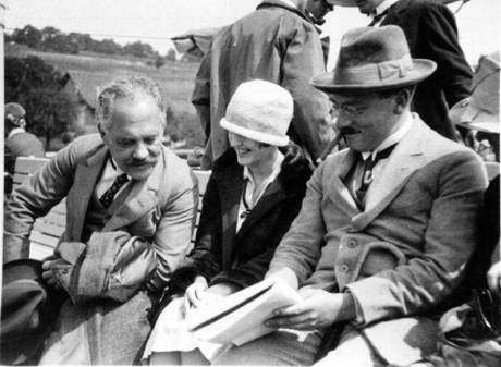
Sommerfeld (l) with Annie Schrödinger, Peter Debye, 1926
...said
"Thermodynamics is a funny subject. The first time you go through it, you don't understand it at all. The second time you go through it, you think you understand it, except for one or two small points. The third time you go through it, you know you don't understand it, but by that time you are so used to it, it doesn't bother you anymore."
Entropy
Our expression for entropy was: $$\begin{align}\frac{S}{k_B} & =\sigma = \ln(w_B) \\ & = \ln N! + \sum_i N_i \ln g_i - \sum_i N_i\ln N_i + \sum_i N_i .\end{align}$$ Now we will find an expression for the middle two terms in the entropy (above):
The 'fished out' equation--*one* of the $n$ Lagrange equations--was $$\ln g_j - \ln N_j +\alpha +\beta E_j = 0.$$
- Multiply by $N_j$:
$$N_j\ln g_j - N_j\ln N_j + \alpha N_j + \beta N_j E_j = 0.$$ - One expression for each $j$. *All* of them are equal to 0. So, adding a bunch of them still gives 0. $$\sum_j N_j\ln g_j - \sum_j N_j\ln N_j +\alpha \sum_j N_j + \beta \sum_j N_j\ E_j = 0.$$
- Two of the sums can be simplified:
$$\sum_j N_j\ln g_j - \sum_j N_j\ln N_j + \alpha N + \beta U = 0.$$ Re-arranging: $$\sum_j N_j\ln g_j - \sum_j N_j\ln N_j = - \alpha N - \beta U$$
Substituting this last expression into the entropy, we get $$\sigma = \ln(w_B) = \ln N! -\alpha N -\beta U + N .$$
Classically, we had: $$T\,dS = dU + P\,dV \Rightarrow dS = \frac{1}{T}dU +\frac{P}{T}dV.$$
If we take $k_B \sigma= k_B \ln w_B = S=S(U,V)$, then this implies $$\begin{align} \frac{1}{T} & = \left( \frac{\partial S}{\partial U} \right)_V = \left( \frac{\partial k_B\ln w_B}{\partial U} \right)_V \\ & = - k_B \beta .\end{align}$$
Ah! This is where $T$ becomes explicit! Apparently:
$$\beta=-\frac{1}{k_BT}.$$
Where does $V$ come into things? $N$ is not a function of $V$. That leaves $g_j=g_j(E_j)$ and $E_j$ itself.  In the case of the particle in the box,
$$E_j = \frac{\pi^2\hbar^2}{2mV^{2/3}}n_j^2.$$
In the case of the particle in the box,
$$E_j = \frac{\pi^2\hbar^2}{2mV^{2/3}}n_j^2.$$
So $E_j$ is a function of $V$, and for partial derivatives, that means holding $V$ constant is the same as holding the energy levels $\left{ E_j \right}$ constant when taking partial derivatives. So, all of the $U$ and $V$ dependence of the entropy is concentrated in the (internal) energy of the system, $U(V,N)$, which also depends on the number of particles.
With $\beta = -1/(kT)$, from the energy level occupancy expression: $$N_j = g_j e^{\alpha}e^{-E_j/(kT)}.$$
The sum over all $j$... $$N = \sum_j^n N_j = e^{\alpha} \sum_j g_j e^{-E_j/(kT)}.$$
So, $e^{\alpha}$ can be written as: $$e^{\alpha} = \frac{N}{\sum_j g_j e^{-E_j/(kT)}}.$$
Now, at last, we can write down that expression for the probability of occupation of a single state using only one Lagrange multiplier (the temperature) in it as:
Boltzmann distribution: expected number of particles per quantum state at equilibrium, for energy level $j$. $$f_j(E_j) = \frac{N_j}{g_j}= e^{\alpha}e^{\beta E_j} =\frac{N e^{-E_j/kT}}{\sum_j g_j e^{-E_j/kT}}.$$
This is the Boltzmann distribution for distinguishable particles: The expected number of particles per quantum state for energy level $j$.
Carter describes it as a "probability" of occupation for any quantum state in level $j$, which is a bit jarring at first because this number can be more than 1. But it's possible to have more than one particle in any given quantum state. So I am calling it the "expected number of particles" instead of a probability.
Solving this for $N_j = f_j g_j$, we find: $$N_j= \frac{N}{Z}g_je^{-E_j/kT}.$$ This is the total expected number of particles in the energy level $j$ at equilibrium.