$\color{red}{\myv E^\parallel_\text{above}}$ $\left(\myv E^\parallel_\text{above}\right)_y$
$\color{red}{\myv E^\parallel_\text{below}}$ $\left(\myv E^\parallel_\text{below}\right)_y$
Boundary conditions
Gauss' law is the most straightforward way to calculate $\myv E$, if parts can be evaluated using symmetry.
If you can't break a problem into pieces solvable by Gauss, the next most productive way of getting to $\myv E$ is often: $$\rho(\myv r')\to V(r)=\frac{1}{4\pi\epsilon_0} \iiint \frac{\rho(\myv r')}{\rr} d \tau' \to - \myv \grad V(\myv r)=\myv E(\myv r).$$
We frequently need to supplement this program with boundary conditions.
Boundary conditions on the electric field
In problem 2.16 (that coaxial cable) the radial component of the electric field had a discontinuity at $s=b$, and it was continuous but "bent" at $s=a$:
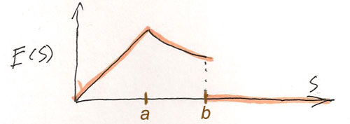
and we know there was some "surface charge" right at $s=b$. Are these observations connected? Yes they are! as we shall now investigate...
Imagine zooming in to a smoothly varying curved surface.
You know that any smoothly curving surface looks "flat" if you zoom in close enough...
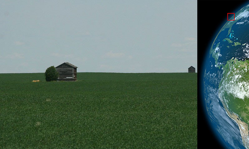
Jeremy Hiebert, Manitoba prairie farmland, and NASA
Furthermore, imagine that the electric field is varying smoothly in the region on either side of a surface. Then when we're sufficiently zoomed in, we would expect that the electric field on either side is approximately constant, but not necessarily equal on either side of the surface.
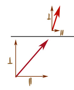
Let's take the approximately constant electric fields on either side of a surface apart into their components parallel and perpendicular to the surface.
Two things to note about this diagram:
- Both of the perpendicular components are parallel to the surface normal direction, let's call it $\uv z$. Therefore they are parallel to each other.
- The components parallel to the surface are both perpendicular to the surface normal $\uv z$, however they are not necessarily mutually parallel.
Components parallel to the surface
The electric field is irrotational, $\myv \grad\times \myv E=0$, which
implies that
path integrals of $\myv E$ are independent of the path taken. This can be expressed as
$$\oint \myv E \cdot d \myv l = 0$$
In this picture, a closed path is shown. Let's say that the parts of the path parallel to the surface are parallel to the $\uv y$ direction.
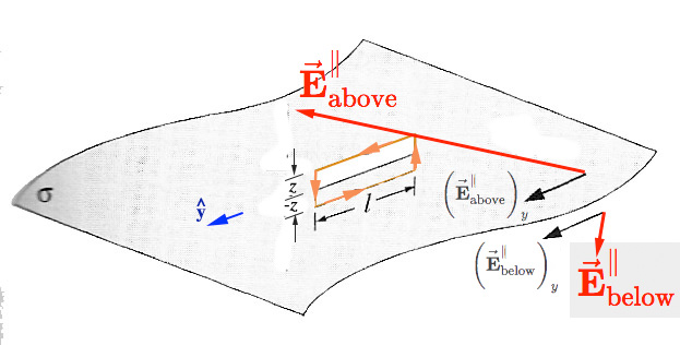
In the limit as the distance, $z$, above / below the surface goes to 0, that line integral has two contributions:
$$\oint \myv E \cdot d\myv l = 0=l\left(E_{\parallel}^\text{above}\right)_y-l\left(E_{\parallel}^\text{below}\right)_y.$$
This implies that $\left(E_{\parallel}^\text{above}\right)_y=\left(E_{\parallel}^\text{below}\right)_y$.
But, we could draw such closed paths in any direction in the plane, and the components of above and below vectors along this direction must be equal for any orientation. This is only possible if $$\Rightarrow \myv E_{\parallel}^\text{above} = \myv E_{\parallel}^\text{below}.$$ So, the component of $\myv E$ that is parallel to the surface must be the same on either side of the surface. That is both the magnitude and the in-plane directions must be the same!
Perpendicular components
Griffiths uses this diagram to think about possible discontinuities in the perpendicular component of the electric field, as you cross a boundary.
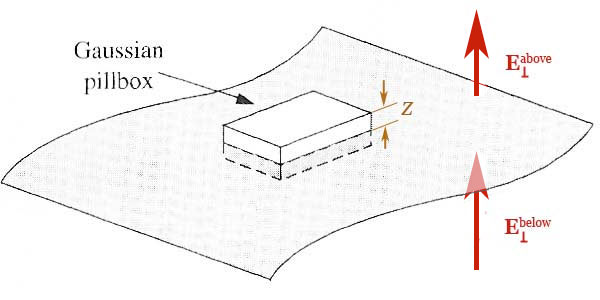
where the top and bottom surface each has area $A$, and they are situated at a height $z$ above (and below) the surface.
We'll apply Gauss' Law $$ \frac{Q_\text{enc}}{\epsilon_0}=\oint_{\cal S}\myv E\cdot d\myv a$$ to the "pillbox" shown:
- Even if there is flux through the side walls, for example due to $\myv E_{\parallel}$, by taking the limit $z\to 0$, the side wall contributions to the flux integral vanish.
- As $z \to 0$, if there is any volume charge density, $\rho$, above or below the surface, those contributions to $Q_\text{enc}$ vanish as well.
- However, if there is a surface charge, $\sigma$, on the surface, it remains as $z\to 0$: So $Q_\text{enc}=\sigma A$.
- Because we're "zoomed in", let us assume that the perpendicular components of $\myv E$ are independent of $x$ and $y$, that is, constant on the top and constant on the bottom surfaces of the pillbox. Then the electric field flux through the top surface (surface normal $\uv z$) is $E^\text{above}_{\perp}A$, and the the flux through the bottom surface (with surface normal $-\uv z$) is $-E^\text{below}_{\perp}A$.
Putting all these considerations together into our Gauss' Law expression: $$\begineq \frac{Q_\text{enc}}{\epsilon_0}&=\oint \myv E\cdot d\myv a\\ \frac{\sigma A}{\epsilon_0}&=E^\text{above}_{\perp}A -E^\text{below}_{\perp}A\\ \frac{\sigma}{\epsilon_0}&=E^\text{above}_{\perp} -E^\text{below}_{\perp} \label{eq:disc} \endeq$$ So the perpendicular component of the electric field is continuous across any surface, unless there is a surface charge on the surface, in which case the discontinuity is proportional to the surface charge density.
Infinite sheet of charge
This result is not in conflict with our result for the electric field of an infinite sheet with a uniform surface charge density, $\sigma$. We found that in this case the electric field was: $$\myv E = \frac{\sigma}{2\epsilon_0}\frac{|z|}{z}\uv{z}$$ That is to say $E^\text{above}_\perp=\frac{\sigma}{2\epsilon_0}$ and $E^\text{below}_{\perp}=-\frac{\sigma }{2\epsilon_0}$. Therefore: $$E^\text{above}_{\perp} -E^\text{below}_{\perp}=\frac{\sigma }{2\epsilon_0} -\left(-\frac{\sigma }{2\epsilon_0}\right) = \frac{\sigma }{\epsilon_0}$$ in agreement with our expression above.
Problem 2.16 (the coaxial cable).
The electric field was in the radial direction, $\uv s$. There was a surface charge density, $\sigma$ at $s=b$, and a discontinuity in the electric field. So, from that problem, take $E_\perp^\text{above}$ to be $E_s^\text{iii}(b)$--that is, the radial component of electric field in region iii, evaluated at $s=b$. And take $E_\perp^\text{below}=E_s^\text{ii}(b)$. Verify that, even though the surface of the coaxial cable is curved, you still get:
$$ E_{\perp}^\text{above} - E_{\perp}^\text{below}=\sigma/\epsilon_0.$$
Remember that the surface charge in this problem exactly cancels out the volume charge in the inner region, such that the $Q_\text{enc} = 0$ for radial distances $s\gt b$.
V is continuous across any boundary
If $\myv a$ is above the surface and $\myv b$ a point below, then the potential difference between these points, as the two points approach other ("$\myv b \leftrightarrow \myv a$") and get closer to the surface is: $$\lim_{\myv b\leftrightarrow \myv a}(V(\myv b)-V(\myv a)) = \lim_{\myv b\leftrightarrow \myv a}\int_{\myv a}^{\myv b} \myv E \cdot d \myv l=0.$$
Of course, that doesn't prevent the gradient from being discontinuous. If '$n$' is the perpendicular distance above the surface, then the discontinuity in the perpendicular component of the electric field shows up in the gradient of the potential as: $$\frac{\del}{\del n}V^\text{above}-\frac{\del}{\del n}V^\text{below} = - \frac{\sigma}{\epsilon_0}$$
Laplace and Poisson differential equations
These two equations... $$\myv E= - \myv \grad V$$ and $$\myv \grad \cdot E= \rho/\epsilon_0,$$
together imply that... $$\Rightarrow \myv \grad \cdot (\myv \grad V) \equiv \grad^2V= -\rho/\epsilon_0.$$
This is known as Poisson's equation.
There are many cases where we're trying to find the field in a region which does not itself contain any charge. So we can restrict ourselves to a special case of Poisson's equation,
Throughout a region without charge, this equation holds:$$\grad^2 V = 0,$$ which has its own name: Laplace's equation.
Summary
Consider a boundary between two regions at $z=0$. The boundary itself might have a surface charge density $\sigma$ [C/m^2] on it...
Examing the electric field, $\color{red}\myv E(\myv r)$, on either side of--above and below--as $z\to 0$, we find...
- The parallel component of the electric field is continuous $$ \myv E_{\parallel}^\text{above} = \myv E_{\parallel}^\text{below}.$$
- The perpendicular component is discontinuous if there is a charge at the interface: $$ \myv E^\text{above}_{\perp} -\myv E^\text{below}_{\perp} = \frac{\sigma}{\epsilon_0}. $$
- The electric potential is continuous $$V^\text{above} = V^\text{below}.$$ But the first derivative, $\frac{\del V}{\del z}$ is not continuous, unless $\sigma=0$.